Get squared Mahalanobis distances to centroid.

For N points, in M dimensions, get squared Mahalanobis distances to center.

mahalDistC(
  m,
  scale = TRUE,
  use = "complete.obs",
  center = c("mean", "median"),
  ...
)

Arguments

m	A data.frame or matrix. Observations in rows.
scale	If TRUE, scale variables before getting mahalanobis distances.
use	Observations to use in computing covariance matrix. Gets passed to cov.
center	Type of univariate center for each variable in m; "mean" or "median"
...	additional arguments passed to mahalanobis, and possibly on to solve.

Value

A list with additional class "mahalDist" containing elements:

1. D2: A vector of squared Mahalanobis distances for observations (rows) in m. Incomplete observations return NA.

2. vars: A character vector with the column names from m.

3. dim: The number of columns of m.

Details

For each of N points in M dimensions, get squared Mahalanobis distances to distribution centroid. This is useful for checking for outliers in a multivariate distribution. The squared Mahalanobis distances to center for an MV normal distribution with N dimensions will follow the chi square distribution with DF equal to N.

This function is a convenience wrapper around mahalanobis, which see. Variables are optionally scaled before distances are computed. Incomplete observations will return NA.

See also

mahalanobis

cov

solve

Author

Dave Braze davebraze@gmail.com

Examples

m <- matrix(rnorm(400, m=.8, s=.05), nrow=100)
md <- mahalDistC(m)
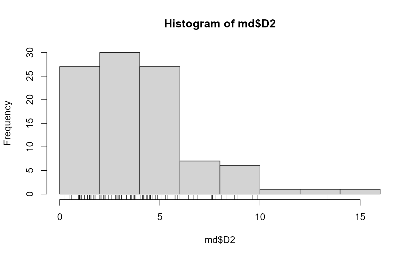
#> [1] -2.492991e-16 -7.763061e-16 -6.873798e-16 -5.496639e-16
md$D2
#>   [1]  6.8657220  0.9967624  2.1921789  5.7690833  1.8006491  1.7996366
#>   [7]  4.1767354  0.9940790  8.0848617  3.7160511  3.5773566  5.1008230
#>  [13] 10.0047741  1.2574886  0.8035108  2.4314170  7.6316181  2.2501739
#>  [19]  0.4695190  2.8496532  3.8011450  4.3806302  3.0917521  5.8855054
#>  [25]  8.8592957  1.5702309  2.8672084  4.8752903  4.6496856  1.4856740
#>  [31]  3.5321995  4.9979474  6.6895551  8.7342380  2.0686514  1.2526548
#>  [37]  3.6983858  2.7532440  5.9997638  4.5340288  1.9777428  2.2642756
#>  [43]  4.5185172  4.4793054  2.2769644  0.5896595  5.7129963  5.2871988
#>  [49]  4.1403004  3.5678466  2.0491749  0.9837629  4.7055502  8.3100221
#>  [55]  6.4275398  2.9227218  1.7204923  1.5474492  1.7109327  5.2980136
#>  [61]  1.0528103  4.2526182  7.5727741  4.3242709  2.7796400  2.8736221
#>  [67]  4.1232919  3.8080036  4.5202648  2.9919090  3.6076073  9.8862185
#>  [73]  2.1013865  2.5960439  9.6141974  7.7916493 14.1958047  1.6203113
#>  [79]  3.7373453  1.2303183  4.7787542  1.7715933  4.0447528  1.3840071
#>  [85]  5.8121648  3.7523112  1.4722260  4.1165165  0.2636546  3.3322626
#>  [91]  1.3903857 13.3903289  4.0103954  1.0912081  5.3714543  0.9328289
#>  [97]  3.5442657  3.0819643  7.0956649  1.6935267
hist(md$D2)
rug(md$D2)